Gridded Population of the World (GPW), v4
Methods
Source Data
Please download the Country-level Information and Sources spreadsheet (Microsoft Excel .xlsx file).
Methods Overview
The methods used to produce the data sets in the GPWv4 collection are described in detail in the formal data collection documentation.
A description of the history of GPW and the development of version 4 is available in Doxsey-Whitfield et al. (2015):
GPWv4 is a minimally-modeled gridded population data collection that incorporates census population data from the 2010 round of censuses. Population estimates are created by extrapolating the raw census counts to estimates for target years 2000, 2005, 2010, 2015, and 2020. Additionally, a set of estimates that have been nationally adjusted to data from the United Nations World Population Prospects 2015 Revision (UN, 2015) is included in the GPWv4 collection for each of the target years. The development of GPWv4 builds upon previous versions of the data collection (Tobler et al., 1997; Deichmann et al., 2001; Balk et al., 2006).
The two basic inputs of GPW are non-spatial population data (i.e., tabular counts of population listed by administrative area) and spatially-explicit administrative boundary data (administrative or enumeration units). Population input data were collected at the highest resolution available from the results of the 2010 round of censuses, which occurred between 2005 and 2014. These were collected from hundreds of national statistics offices and other organizations. Where census results were unavailable or not yet released, official population estimates from national statistical offices or the United Nations were used. Administrative boundary data were collected from a variety of national agencies (e.g. statistics offices, mapping agencies, planning agencies), as well as other organizations, , such as humanitarian agencies (e.g., U.N. OCHA). Ideally, the boundaries for a given country were those originating with the census. In the absence of official census boundaries, other administrative boundary data were used. The population census counts or official estimates were then matched to digital geographic boundaries. Matching was based on the common identifying codes or the unit names used in the census.
A global framework of international boundaries was used to ensure consistent alignment between countries. The Global Administrative Areas version 2 (GADMv2; www.gadm.org) data set was selected as the framework as it is publicly available and frequently used in the research community. The international boundaries of census geography data sets were adjusted to the GADMv2 framework, although in cases where the resolution of the census geography far exceeded the GADMv2 boundaries, the former were kept (e.g., New Zealand, the United Kingdom, and the United States).
To facilitate global comparison of countries that conduct their censuses at different times, annualized growth rates were used to estimate counts for the target years of 2000, 2005, 2010, 2015, and 2020. Growth rates were calculated for each administrative unit by matching to a previous census enumeration or estimate. Annualized rates of change were calculated as follows:
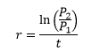
where r is the annualized growth rate, P1 and P2 are the census population counts, Px is the population estimate in the target year, and t is the number of years between population counts.
Population estimates were then calculated for the target years as follows:
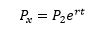
where Px is the population estimate in the target year x, and P2, r and t are as defined above.
For some countries, it was not possible to match at the highest resolution between the two points in time. For these countries, censuses were matched and growth rates were calculated at a coarser resolution (e.g., state), and applied to each nested higher resolution unit (e.g., county). In some cases we adopted a hybrid approach, matching the highest resolution where possible and coarsening where needed. The 2010 population estimates were then extrapolated to 2000, 2005, 2015, and 2020 using the calculated annualized growth rates.
The National-level estimates for 2000, 2005, 2010, 2015, and 2020 were the adjusted to the estimates of the United Nation’s World Population Prospects (WPP): The 2015 Revision (United Nations, 2015).
Adjustment factors for matching national estimates to UN estimates are calculated as follows:
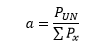
where a is the adjustment factor, Px is the population estimate in the target year, PUN is the UN national estimate for the target year.
Adjustment factors were applied at the sub-national level as follows:
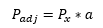
where Padj is the sub-national UNWPP-adjusted estimate, and Px and a are as defined above.
In order to achieve full global coverage of cross-tabulated age by sex population count estimates, it was necessary to consult a variety of source data. These data are predominantly census based and at the same geographic scale as the total population count data. There are, however, a number of countries for which cross-tabulated variables were only available from alternative sources or at coarser geographic scales.
The estimation of the demographic variables, age and sex, was accomplished through the following procedure.
First, if single-year age data were available for a given country, the data were aggregated into 5-year age groups.
Second, estimates of the male and female population in 2010 were created by calculating the proportions of males and females in each geographic unit for the year of the input data, and applying those proportions to the 2010 estimates of total population for each unit, as follows:
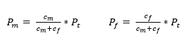 where P is the 2010 estimated population, c is the census population, and the subscripts m, f, and t refer to male, female, and total, respectively.
Third, estimates of the population by age and sex in 2010 were created by calculating the proportions of males and females in each 5-year age group for each geographic unit for the year of the input data, and applying those proportions to the 2010 estimates of male and female population calculated in step one, as follows:
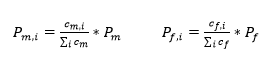 where the subscript i refers to any age group in the set of all age groups, and P, c, m, and f are as defined above.
Fourth, five maximum age group classes were calculated from the age estimates: 65+, 70+, 75+, 80+, and 85+. Each of these classes was only calculated for countries with available data. The highest age group class with global coverage is 65+.
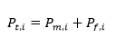
Finally, the corresponding male and female age groups were summed to produce the estimated total population in that age group for year 2010:
 Four countries (Benin, Loas, Malaysia, and Sri Lanka) required additional pre-processing in order to produce high resolution cross-tabulated variable estimates. Details can be found in the Methods section of the GPWv4 documentation pdf.
To create the raster population data sets, the population estimates were distributed to a 30 arc-second (~1 km at the equator) grid using an areal-weighting method. This method, also known as uniform distribution or proportional allocation, does not make use of any other geographic data in order to spatially disaggregate the census population. Population was allocated to the raster pixels (i.e., grid cells) through the simple assumption that the population of a pixel is the exclusive function of the land area within that pixel. For pixels that intersect sub-national or national boundaries, population was allocated based on the proportion of the area. A water mask was applied to the data to prevent lakes, rivers, and ice-covered areas from distorting the actual population distribution.
In addition, the native 30 arc-second resolution data were aggregated to four lower resolutions (2.5 arc-minute, 15 arc-minute, 30 arc-minute, and 1 degree) to enable faster global processing and support research communities that conduct analyses at these resolutions. Table 1 provides unit equivalents for these different cell sizes. All spatial data sets in the GPWv4 collection are stored in geographic coordinate system (latitude/longitude).

References
Balk, D.L., U. Deichmann, G. Yetman, F. Pozzi, S.I. Hay, and A. Nelson. 2006. Determining global population distribution: methods, applications and data. Advances in Parasitology 62:119-156. https://doi.org/10.1016/S0065-308X(05)62004-0.
Deichmann, U., D. Balk, and G. Yetman. 2001. Transforming Population Data for Interdisciplinary Usages: From Census to Grid. Palisades, NY: NASA Socioeconomic Data and Applications Center (SEDAC), CIESIN, Columbia University. http://sedac.ciesin.columbia.edu/downloads/docs/gpw-v3/gpwdocumentation.pdf.
Doxsey-Whitfield, E., K. MacManus, S.B. Adamo, L. Pistolesi, J. Squires, O. Borkovska, and S.R. Baptista. 2015. Taking advantage of the improved availability of census data: A first look at the Gridded Population of the World, Version 4 (GPWv4). Papers in Applied Geography 1(3): 226-234. https://doi.org/10.1080/23754931.2015.1014272.
Tobler, W., U. Deichmann, J. Gottsegen, and K. Maloy. 1997. World population in a grid of spherical quadrilaterals. International Journal of Population Geography 3:203-225. https://doi.org/10.1002/(SICI)1099-1220(199709)3:3<203::AID-IJPG68>3.0.CO;2-C.
United Nations, Department of Economic and Social Affairs, Population Division (2015). World Population Prospects: The 2015 Revision, DVD Edition. http://esa.un.org/unpd/wpp/DVD/.